RND (Random Network Distillation) with Proximal Policy Optimization (PPO) Tensorflow

This post documents my implementation of the Random Network Distillation (RND) with Proximal Policy Optimization (PPO) algorithm. (continuous version)

Random Network Distillation (RND) with Proximal Policy Optimization (PPO) implentation in Tensorflow. This is a continuous version which solves the mountain car continuous problem (MountainCarContinuous-v0). The RND helps learning with curiosity driven exploration.

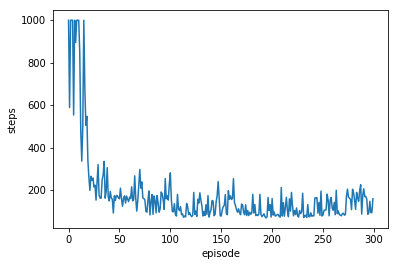
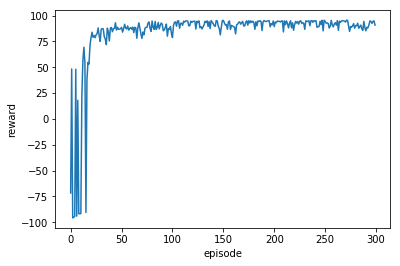
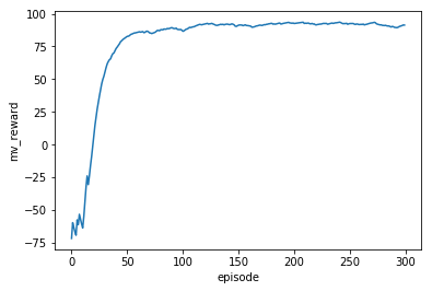
The agent starts to converge correctly at around 30 episodes & reached the flag 291 times out of 300 episodes (97% hit rate). It takes 385.09387278556824 seconds to complete 300 episodes on Google’s Colab.

Edit: A new version which corrects a numerical error(causes nan action) takes 780.2065596580505 seconds for 300 episodes. Both versions have similar results. The URL for the new version is updated. Added random seeds for numpy & Tensorflow global seed & ops seed achieve better consistency & faster convergence.

Checkout the resulting charts from the program output.

Code on my Github:

• Python file,

• Jupyter notebook (The Jupyter notebook, which also contain the resulting charts at the end, can be run directly on Google’s Colab.)

If Github is not loading the Jupyter notebook, a known Github issue, click here to view the notebook on Jupyter’s nbviewer.

Notations & equations

fixed feature from target network = \({ f (s_{t+1}) }\)

predicted feature from predictor network = \({ f ^\prime (s_{t+1}) }\)

intrinsic reward = \(r_{i}\) = || \({ f ^\prime (s_{t+1}) }\) - \({ f (s_{t+1}) }\) || \({}{^2}\)

For notations & equations regarding PPO, refer to this post.

Key implementation details:

Preprocessing, state featurization:

Prior to training, the states are featurized with the RBF kernel.

(states are also featurized during every training batch.)

Refer to scikit-learn.org documentation: 5.7.2. Radial Basis Function Kernel for more information on RBF kernel.

if state_ftr == True:
"""
The following code for state featurization is adapted & modified from dennybritz's repository located at:
https://github.com/dennybritz/reinforcement-learning/blob/master/PolicyGradient/Continuous%20MountainCar%20Actor%20Critic%20Solution.ipynb
"""
    # Feature Preprocessing: Normalize to zero mean and unit variance
    # We use a few samples from the observation space to do this
    states = np.array([env.observation_space.sample() for x in range(sample_size)]) # pre-trained, states preprocessing
    scaler = sklearn.preprocessing.StandardScaler()
    scaler.fit(states) # Compute the mean and std to be used for later scaling.

    # convert states to a featurizes representation.
    # We use RBF kernels with different variances to cover different parts of the space
    featurizer = sklearn.pipeline.FeatureUnion([ # Concatenates results of multiple transformer objects.
            ("rbf1", RBFSampler(gamma=5.0, n_components=n_comp)),
            ("rbf2", RBFSampler(gamma=2.0, n_components=n_comp)),
            ("rbf3", RBFSampler(gamma=1.0, n_components=n_comp)),
            ("rbf4", RBFSampler(gamma=0.5, n_components=n_comp))
            ])
    featurizer.fit(
        scaler.transform(states)) # Perform standardization by centering and scaling

# state featurization of state(s) only,
# not used on s_ for RND's target & predictor networks
def featurize_state(state):
    scaled = scaler.transform([state]) # Perform standardization by centering and scaling
    featurized = featurizer.transform(scaled) # Transform X separately by each transformer, concatenate results.
    return featurized[0]

def featurize_batch_state(batch_states):
    fs_list = []
    for s in batch_states:
        fs = featurize_state(s)
        fs_list.append(fs)
    return fs_list

Preprocessing, next state normalization for RND:

Variance is computed for the next states buffer_s_ using the RunningStats class. During every training batch, the next states are normalize and clipped.

def state_next_normalize(sample_size, running_stats_s_):

  buffer_s_ = []
  s = env.reset()
  for i in range(sample_size):
    a = env.action_space.sample()
    s_, r, done, _ = env.step(a)
    buffer_s_.append(s_)

  running_stats_s_.update(np.array(buffer_s_))

if state_next_normal == True:
  state_next_normalize(sample_size, running_stats_s_)

Tensorboard graphs:

Big picture:

There are two main modules, the PPO and the RND.

Current state, state is passed into PPO.

Next state, state_ is passed into RND.

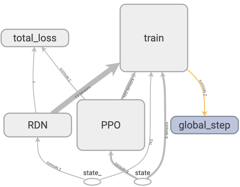
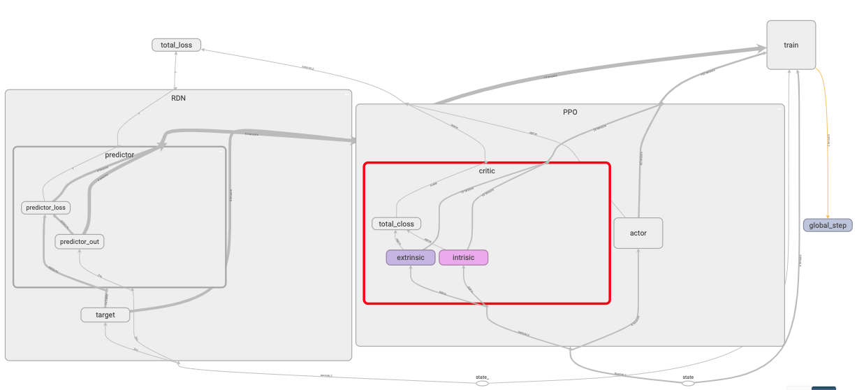
PPO module:

PPO module contains the actor network & the critic network.

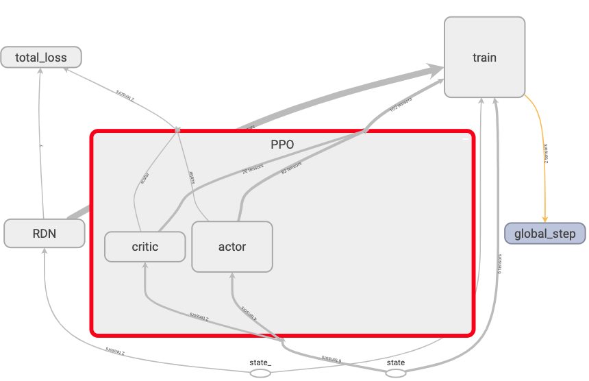
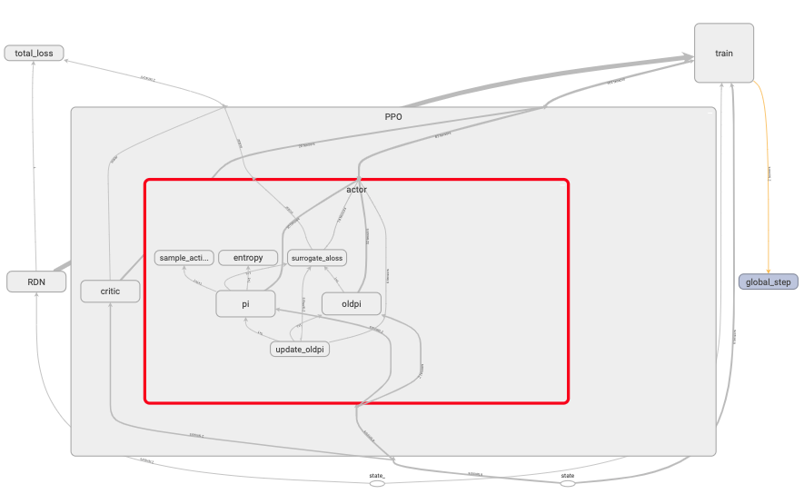
PPO’s actor:

At every iteration, an action is sampled from policy network pi.

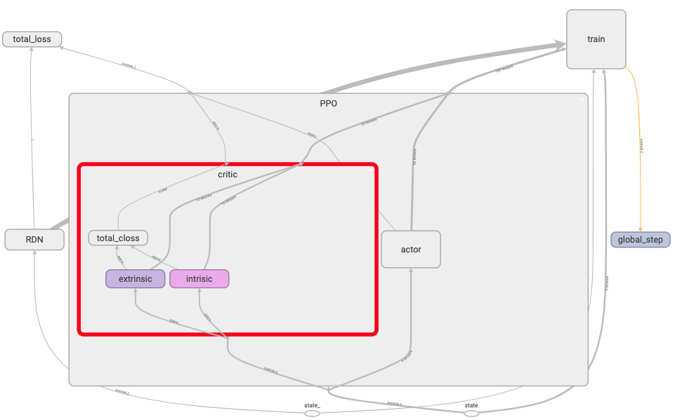
PPO’s critic:

The critic contains two value function networks. One for extrinsic rewards & one for intrinsic rewards. Two sets of TD lambda returns & advantages are also computed.

For extrinsic rewards: tdlamret adv

For intrinsic rewards: tdlamret_i adv_i

The TD lambda returns are used as the PPO’s critics targets in their respective networks while the advantages are summed & used as the advantage in the actor’s loss computation.

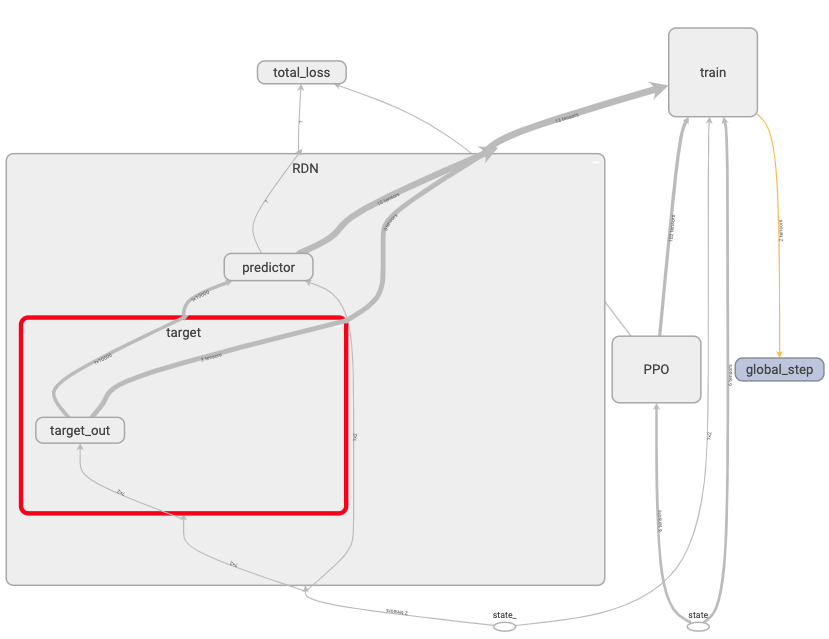
RND module:

RND module contains the target network & the predictor network.

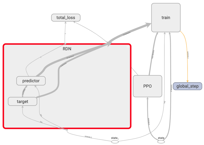
RND target network:

The target network is a fixed network, meaning that it’s never trained. It’s weights are randomized once during initialization. The target network is used to encode next states state_. It’s output are encoded next states.

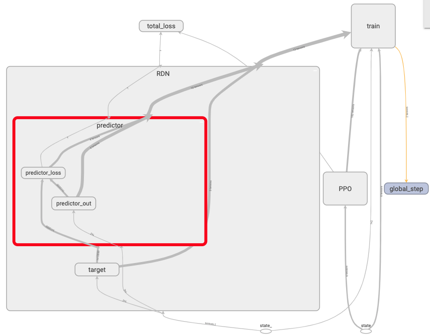
RND predictor network:

The predictor_loss is the intrinsic reward. It is the difference between the predictor network’s output with the target network’s output. The predictor network is trying to guess the target network’s encoded output.

Key to note:

All networks used in this program are linear.

The actor module is basically similar to this DPPO code documented in this post.

The difference is in the critic module. This implementation has two value functions in the critic module rather than one.

The predictor_loss is the intrinsic reward.

Problems encountered:

The actor’s network occasionally returns ‘'’nan’’’ for action. This happens randomly, most likely caused by exploding gradients. Not initializing or randomly initializing actor’s weights results in nan when outputting action.

Program output:

hit_counter 291 0.97

Number of steps per episode:

Reward per episode:

Moving average reward per episode:

— 385.09387278556824 seconds —

References:

Exploration by Random Network Distillation (Yuri Burda, Harrison Edwards, Amos Storkey, Oleg Klimov, 2018)

• 2020 10
• 2019 24