Measurement & mixed states for quantum systems.
Notes on measurement for quantum systems.
A custom MARL (multi-agent reinforcement learning) environment where multiple agents trade against one another in a CDA (continuous double auction).
This is WIP.
Code on my Github
1) Update
3) Example
4) Dependencies
5) Installation
6) TODO
8) Contributing
9) Disclaimer
11) Action space
12) Making sense of the render output
13) Generated LOB
20200612
1) Breakup training script into smaller parts under train folder.
2) Some info from trader’s account such as NAV are added to the environment’s step info dictionary.
3) Added logging/loading of step & episodic data to json files with gzip.
4) Added subplot functionalities for self-play generated LOB data.
The purpose of this repository is to create a custom MARL (multi-agent reinforcement learning) environment where multiple agents trade against one another in a CDA (continuous double auction).
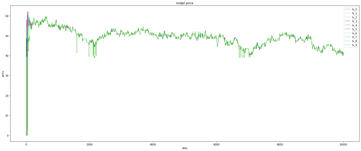
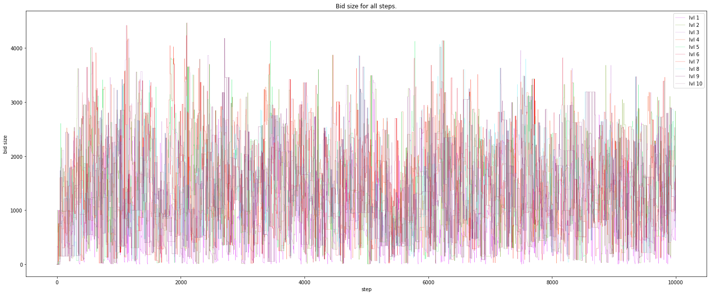
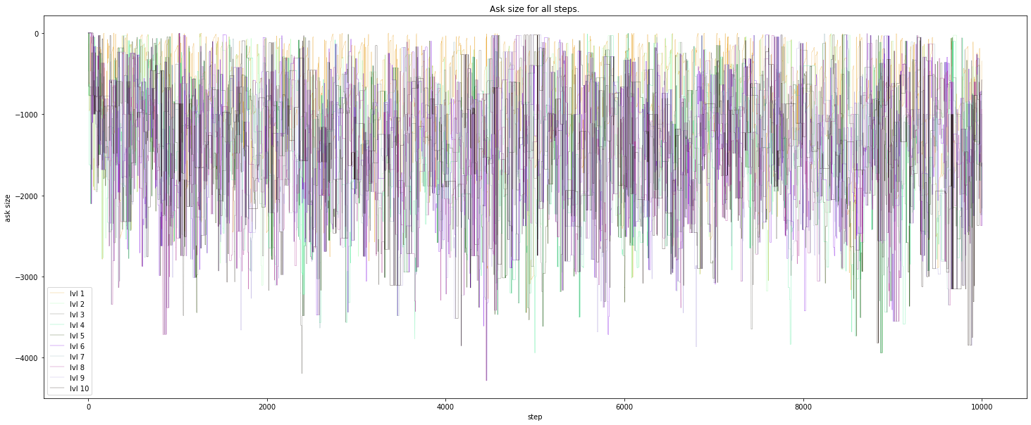
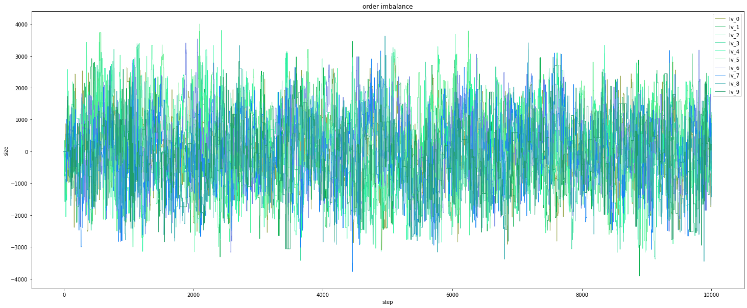
The environment doesn’t use any external data. Data is generated by self-play of the agents themselves through their interaction with the limit order book.
At each time step, the environment emits the top k rows of the aggregated order book as observations to the agents. Each agent then samples an action from the action space & all actions are randomly shuffled before execution in each time step.
Each time step is a snapshot of the limit order book & a key assumption is that all traders(agents) suffer the same lag (wait for all traders to have their orders executed before seeing the next LOB snapshot).
The example is available in this Jupyter notebook implemented with
RLlib: CDA_env_RLlib_NSF.ipynb. This notebook is tested in Colab.
This example uses two trained agents & N random agents. All agents compete with one another in this zero-sum environment, irregardless of whether they’re trained or random.
competitive self-play
The policy weights of the winning trained agent(trader) is used to replace the policy weights of the other trained agents after each training iteration. Winning here is defined as having the highest reward per training iteration.
The reward function requires the agents to maximize profit while minimizing number of trades made in an episode (trading session). As the number of trades accumulates in the later stages of a session, profits will be scaled down by the number of trades & losses will be magnified.
The trained agents are P0 & P1, both using separate PPO policy weights. The rest are random agents.
The results with 10 agents are shown in the figures below:
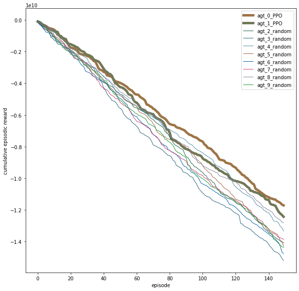
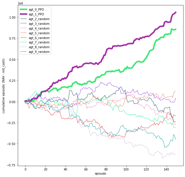
If you’re running locally, you can run the following command & navigate
to localhost:6006 in your browser to access the tensorboard graphs:
$ tensorboard --logdir ~/ray_results
Other ways to run this environment:
By using the python CDA_env_rand.py script which is basically running a
CDA simulator with dummy (non-learning) random agents.
1) tensorFlow
2) ray[rllib]
3) pandas
4) sortedcontainers
5) sklearn
For a full list of dependencies & versions, see requirements.txt in this
repository.
The environment is installable via pip.
$ cd gym-continuousDoubleAuction

$ pip install -e .
1) Better documentation.
2) More robust tests (add LOB test into test script).
3) Generalize the environment to use more than 1 LOB.
4) Parametric or hybrid action space (or experiment with different types of action space).
5) Expose the limit orders (that are currently in the LOB or aggregated LOB) which belongs to a particular trader as observation to that trader.
6) Allow traders to have random starting capital.
7) Instead of traders(agents) having the same lag, introduce zero lag (Each LOB snapshot in each t-step is visible to all traders) or random lag.
8) Allows a distribution of previous winning policies to be selected for trained agents (for training script).
9) Custom RLlib workflow to include custom RND + PPO policies (for training script).
10) Update current sample model (deprecated) (for training script).
11) Move TODO to issues.
The orderbook matching engine is adapted from https://github.com/dyn4mik3/OrderBook
Please see CONTRIBUTING.md.
This repository is only meant for research purposes & is never meant to be used in any form of trading. Past performance is no guarantee of future results. If you suffer losses from using this repository, you are the sole person responsible for the losses. The author will NOT be held responsible in any way.
Each obs is a snapshot in each environment step.
obs = [array([1026., 2883., 1258., 1263., 3392., 1300., 1950., 1894., 2401., 4241.],          # bid size list
       array([64., 63., 62., 61., 60., 59., 58., 57., 56., 55.]),                             # bid price list
       array([ -519., -2108.,  -215., -1094., -1687., -2667., -3440., -2902., -1440 -3078.]), # ask size list
       array([-65., -66., -67., -68., -69., -70., -71., -72., -73., -74.])]                   # ask price list
See PR 9 for the current action space.
The step separator:
************************************************** t_step = 306 **************************************************
Actions:
Actions output from the model:
1) Each column represents the action from each trader(agent).
2) Row 1 represents the side: none, bid, ask (0 to 2).
3) Row 2 represents the type: market, limit, modify, cancel.
4) Row 3 represents the mean for size selection.
5) Row 4 represents the sigma for size selection.
6) Row 5 represents the price: based on LOB market depth from 0 to 11.
Model actions:
 --  --  --  --
 1   1   1   2
 1   0   0   1
39  29   6  17
19  89  13   0
 7   4   9  10
--  --  --  --
1) Column 1 represents the ID of each trader(agent).
2) Column 2 the side: none, bid, ask (0 to 2).
3) Column 3 type: market, limit, modify, cancel.
4) Column 4 represents the order size.
5) Column 5 represents the order price.
Formatted actions acceptable by LOB:
 -  ---  ------  -----  --
0  bid  limit   38982  15
1  bid  market   5779   0
2  bid  market    999   0
3  ask  limit   17001  47
-  ---  ------  -----  --
Shuffled action queue sequence for LOB executions:
 -  ---  ------  -----  --
3  ask  limit   17001  47
2  bid  market    999   0
1  bid  market   5779   0
0  bid  limit   38982  15
-  ---  ------  -----  --
Rewards, dones, & infos:
rewards:
 {0: 0.0, 1: 0.0, 2: 0.0, 3: 0.0}

dones:
 {'__all__': True}

infos:
 {0: {}, 1: {}, 2: {}, 3: {}}
Aggregated LOB:
1) The columns represents the 10 levels (1 to 10, left to right) of the market depth in the LOB.
2) Row 1 represents the bid size.
3) Row 2 represents the bid price.
4) Row 3 represents the ask size.
5) Row 4 represents the ask price.
agg LOB @ t-1
 ------  -----  ------  ------  ------  ------  ------  ------  ------  ------
  7746  19011  126634  116130   43073  124055   74977  188096  139117  143968
    23     22      21      20      19      15      14      12      11      10
-62448  -7224  -65989  -96940  -77985  -93987  -55942   -4173  -16998  -81011
   -36    -37     -38     -39     -40     -41     -42     -43     -47     -48
------  -----  ------  ------  ------  ------  ------  ------  ------  ------
agg LOB @ t
 ------  -----  ------  ------  ------  ------  ------  ------  ------  ------
  7746  19011  126634  116130   43073  163037   74977  188096  139117  143968
    23     22      21      20      19      15      14      12      11      10
-56669  -7224  -65989  -96940  -77985  -93987  -55942   -4173  -33999  -81011
   -36    -37     -38     -39     -40     -41     -42     -43     -47     -48
------  -----  ------  ------  ------  ------  ------  ------  ------  ------
LOB bids:
The current limit bid orders in the LOB.
LOB:
 ***Bids***
     size price  trade_id  timestamp  order_id
0    7746    23         0        345       265
1   19011    22         1        344       231
2   14553    21         2        107        99
3   63025    21         1        333       209
4   49056    21         3        349       268
5   89029    20         2         53        53
6   24060    20         0        201        46
7    3041    20         1        297       229
8   43073    19         1         35        35
9   42989    15         1        340       234
10  81066    15         3        336       259
11  38982    15         0        359       275
12  63003    14         0        253       201
13  11974    14         1        285       168
14  18089    12         3        351       105
15  91998    12         0        343       264
16  78009    12         1        352        40
17  45039    11         3        123       101
18  94078    11         0        204       172
19  97967    10         3        223       185
20  46001    10         1        313       243
21  45871     9         2         52        52
22  94993     9         3        209       176
LOB asks:
The current limit ask orders in the LOB.
***Asks***
     size price  trade_id  timestamp  order_id
0   40654    36         3        322       250
1   16015    36         0        323       251
2    7224    37         1        272       214
3   39980    38         3        299       190
4   26009    38         1        261       206
5   58977    39         0        231       188
6   37963    39         3        284       164
7   15995    40         0        305       235
8   61990    40         3        328       254
9   93987    41         0        353       143
10  55942    42         1        290       189
11   4173    43         0        112       104
12  16998    47         1        341       239
Tape (Time & sales):
***tape***
    size price  timestamp  counter_party_ID  init_party_ID init_party_side
0   5779    36        358                 3              1             bid
1   5894    36        356                 3              0             bid
2  13347    36        355                 3              1             bid
3   2272    36        354                 3              0             bid
4    894    23        350                 0              1             ask
5  12874    23        347                 0              0             ask
6   7501    23        346                 0              1             ask
7   9405    22        342                 1              3             ask
Trades:
Trades that took place when executing the action of a trader(agent) at t-step.
act_seq_num represents the sequence of the action. In this case, it’s the 2nd action executed at t-step.
TRADES (act_seq_num): 2
   seq_Trade_ID  timestamp price    size  time  counter_ID counter_side  counter_order_ID counter_new_book_size  init_ID init_side init_order_ID init_new_LOB_size
0             0        358    36  5779.0   358           3          ask               250                 40654        1       bid          None              None
New order in LOB:
The new limit orders inserted into LOB (includes unfilled leftover quantity from previous order).
order_in_book (act_seq_num): 0
type    side      quantity    price    trade_id    timestamp    order_id
------  ------  ----------  -------  ----------  -----------  ----------
limit   ask          17001       47           3          357         273
order_in_book (act_seq_num): 3
type    side      quantity    price    trade_id    timestamp    order_id
------  ------  ----------  -------  ----------  -----------  ----------
limit   bid          38982       15           0          359         275
Mark to market profit @ t-step:
mark_to_mkt profit@t:
ID: 0; profit: 1491150.999999999999999999998
ID: 1; profit: 3583508.999999999999999999995
ID: 2; profit: -7421583.999999999999999999999
ID: 3; profit: -676658.0000000000000000000013
Accounts info:
Accounts:
   ID          cash    cash_on_hold    position_val      prev_nav           nav    net_position     VWAP             profit    total_profit    num_trades
----  ------------  --------------  --------------  ------------  ------------  --------------  -------  -----------------  --------------  ------------
   0  -4.51044e+07     3.11089e+07     1.64866e+07   2.49115e+06   2.49115e+06         -375119  39.9751        1.49115e+06     1.49115e+06            74
   1  -3.8919e+07      3.27787e+07     1.07237e+07   4.58351e+06   4.58351e+06          -98798  72.2711        3.58351e+06     3.58351e+06            78
   2  -1.92421e+07     3.55094e+06     9.2696e+06   -6.42158e+06  -6.42158e+06          257489  64.8229       -7.42158e+06    -7.42158e+06            23
   3  -4.46985e+07     4.0254e+07      7.79141e+06   3.34692e+06   3.34692e+06          216428  39.1265  -676658               2.34692e+06            79
1) total_sys_profit (total profit of all agents at each step) should be equal to 0 (zero-sum game).
2) total_sys_nav (total net asset value of all agents at each step) is the total sum of beginning NAV of all traders(agents).
Note: Small random rounding errors are present.
total_sys_profit = -9E-21; total_sys_nav = 3999999.999999999999999999991
Sample output results for final training iteration:
1) The episode_reward is zero (zero sum game) for each episode.
episode_reward_max: 0.0
episode_reward_mean: 0.0
episode_reward_min: 0.0
2) The mean reward of each policy is shown under policy_reward_mean.
.
.
.
Result for PPO_continuousDoubleAuction-v0_0:
custom_metrics: {}
date: 2019-09-30_21-16-20
done: true
episode_len_mean: 1001.0
episode_reward_max: 0.0
episode_reward_mean: 0.0
episode_reward_min: 0.0
episodes_this_iter: 4
episodes_total: 38
experiment_id: 56cbdad4389343eca5cfd49eadeb3554
hostname: Duality0.local
info:
grad_time_ms: 15007.219
learner:
policy_0:
cur_kl_coeff: 0.0003906250058207661
cur_lr: 4.999999873689376e-05
entropy: 10.819798469543457
entropy_coeff: 0.0
kl: 8.689265087014064e-06
model: {}
policy_loss: 153.9163055419922
total_loss: 843138688.0
vf_explained_var: 0.0
vf_loss: 843138496.0
num_steps_sampled: 40000
num_steps_trained: 40000
opt_peak_throughput: 266.538
opt_samples: 4000.0
sample_peak_throughput: 80.462
sample_time_ms: 49713.208
update_time_ms: 176.14
iterations_since_restore: 10
node_ip: 192.168.1.12
num_healthy_workers: 2
off_policy_estimator: {}
pid: 10220
policy_reward_mean:
policy_0: 12414.421052631578
policy_1: -301.39473684210526
policy_2: -952.1578947368421
policy_3: -11160.868421052632
sampler_perf:
mean_env_wait_ms: 18.1753569144153
mean_inference_ms: 4.126144958830859
mean_processing_ms: 1.5262831265657335
time_since_restore: 649.1416146755219
time_this_iter_s: 61.54709506034851
time_total_s: 649.1416146755219
timestamp: 1569849380
timesteps_since_restore: 40000
timesteps_this_iter: 4000
timesteps_total: 40000
training_iteration: 10
trial_id: ea67f638
2019-09-30 21:16:20,507 WARNING util.py:145 -- The `process_trial` operation took 0.4397752285003662 seconds to complete, which may be a performance bottleneck.
2019-09-30 21:16:21,407 WARNING util.py:145 -- The `experiment_checkpoint` operation took 0.899777889251709 seconds to complete, which may be a performance bottleneck.
== Status ==
Using FIFO scheduling algorithm.
Resources requested: 0/4 CPUs, 0/0 GPUs
Memory usage on this node: 3.3/4.3 GB
Result logdir: /Users/hadron0/ray_results/PPO
Number of trials: 1 ({'TERMINATED': 1})
TERMINATED trials:
- PPO_continuousDoubleAuction-v0_0: TERMINATED, [3 CPUs, 0 GPUs], [pid=10220], 649 s, 10 iter, 40000 ts, 0 rew
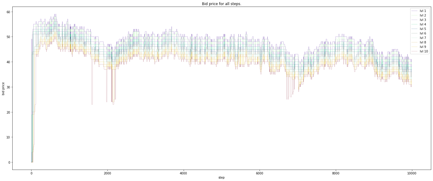
Bid price:
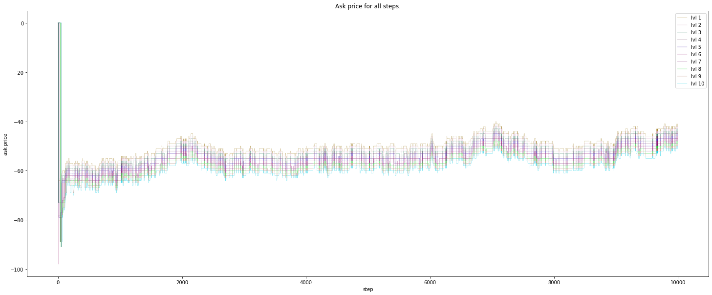
Ask price:
Midpoint price:
Bid size:
Ask size:
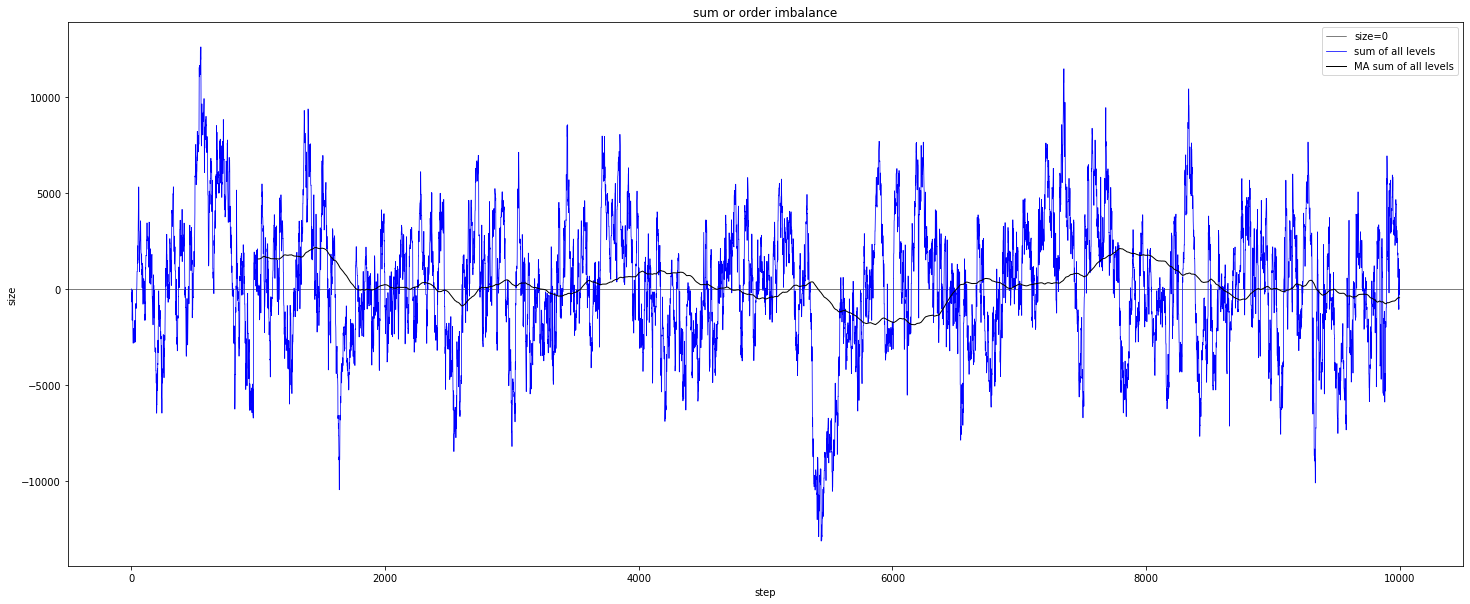
Order imbalance:
Sum of order imbalance:
Notes on measurement for quantum systems.
Notes on quantum states as a generalization of classical probabilities.
The location of ray_results folder in colab when using RLlib &/or tune.
My attempt to implement a water down version of PBT (Population based training) for MARL (Multi-agent reinforcement learning).
Ray (0.8.2) RLlib trainer common config from:
How to calculate dimension of output from a convolution layer?
Changing Google drive directory in Colab.
Notes on the probability for linear regression (Bayesian)
Notes on the math for RNN back propagation through time(BPTT), part 2. The 1st derivative of \(h_t\) with respect to \(h_{t-1}\).
Notes on the math for RNN back propagation through time(BPTT).
Filter rows with same column values in a Pandas dataframe.
Building & testing custom Sagemaker RL container.
Demo setup for simple (reinforcement learning) custom environment in Sagemaker. This example uses Proximal Policy Optimization with Ray (RLlib).
Basic workflow of testing a Django & Postgres web app with Travis (continuous integration) & deployment to Heroku (continuous deployment).
Basic workflow of testing a dockerized Django & Postgres web app with Travis (continuous integration) & deployment to Heroku (continuous deployment).
Introducing a delay to allow proper connection between dockerized Postgres & Django web app in Travis CI.
Creating & seeding a random policy class in RLlib.
A custom MARL (multi-agent reinforcement learning) environment where multiple agents trade against one another in a CDA (continuous double auction).
This post demonstrate how setup & access Tensorflow graphs.
This post demonstrates how to create customized functions to bundle commands in a .bash_profile file on Mac.
This post documents my implementation of the Random Network Distillation (RND) with Proximal Policy Optimization (PPO) algorithm. (continuous version)
This post documents my implementation of the Distributed Proximal Policy Optimization (Distributed PPO or DPPO) algorithm. (Distributed continuous version)
This post documents my implementation of the A3C (Asynchronous Advantage Actor Critic) algorithm (Distributed discrete version).
This post documents my implementation of the A3C (Asynchronous Advantage Actor Critic) algorithm. (multi-threaded continuous version)
This post documents my implementation of the A3C (Asynchronous Advantage Actor Critic) algorithm (discrete). (multi-threaded discrete version)
This post demonstrates how to accumulate gradients with Tensorflow.
This post demonstrates a simple usage example of distributed Tensorflow with Python multiprocessing package.
This post documents my implementation of the N-step Q-values estimation algorithm.
This post demonstrates how to use the Python’s multiprocessing package to achieve parallel data generation.
This post provides a simple usage examples for common Numpy array manipulation.
This post documents my implementation of the Dueling Double Deep Q Network with Priority Experience Replay (Duel DDQN with PER) algorithm.
This post documents my implementation of the Dueling Double Deep Q Network (Dueling DDQN) algorithm.
This post documents my implementation of the Double Deep Q Network (DDQN) algorithm.
This post documents my implementation of the Deep Q Network (DQN) algorithm.