A3C multi-threaded discrete version with N step targets

This post documents my implementation of the A3C (Asynchronous Advantage Actor Critic) algorithm (discrete). (multi-threaded discrete version)

A3C (Asynchronous Advantage Actor Critic) implementation with Tensorflow. This is a multi-threaded discrete version. The code is tested with Gym’s discrete action space environment, CartPole-v0 on Colab.

Code on my Github: (missing terms are treated as 0)

If Github is not loading the Jupyter notebook, a known Github issue, click here to view the notebook on Jupyter’s nbviewer.

Code on my Github: (use maximum terms possible)

If Github is not loading the Jupyter notebook, a known Github issue, click here to view the notebook on Jupyter’s nbviewer.

Notations:

Actor network = \({\pi}_{\theta}\)

Actor network parameter = \({\theta}\)

Critic network = \(V_{\phi}\)

Critic network parameter = \(\phi\)

Advantage function = A

Number of trajectories = m

Equations:

Actor component: log\({\pi}_{\theta}\) \((a_{t} {\mid} s_{t})\)

Critic component = Advantage function = A = \(Q(s_{t}, a_{t})\) - \(V_{\phi}(s_{t})\)

Q values with N-step truncated estimate :

\(Q^{\pi}(s_{t}, a_{t})\) = E(\(r_{t}\) + \(\gamma\) \(r_{t+1}\) + \(\gamma^{2}\) \(r_{t+2}\) + … + \(\gamma^{n}\) V(\(s_{t+n}\)))

Check this post for more information on N-step truncated estimate.

Policy gradient estimator

= \(\nabla_\theta J(\theta)\)

= \({\dfrac{1}{m}}\) \({\sum\limits_{i=1}^{m}}\) \({\sum\limits_{t=0}^{T}}\) \(\nabla_\theta\) log\({\pi}_{\theta}\) \((a_{t} {\mid} s_{t})\) \(Q(s_{t}, a_{t})\) - \(V_{\phi}(s_{t})\)

= \({\dfrac{1}{m}}\) \({\sum\limits_{i=1}^{m}}\) \({\sum\limits_{t=0}^{T}}\) \(\nabla_\theta\) log\({\pi}_{\theta}\) \((a_{t} {\mid} s_{t})\) A

Key implementation details:

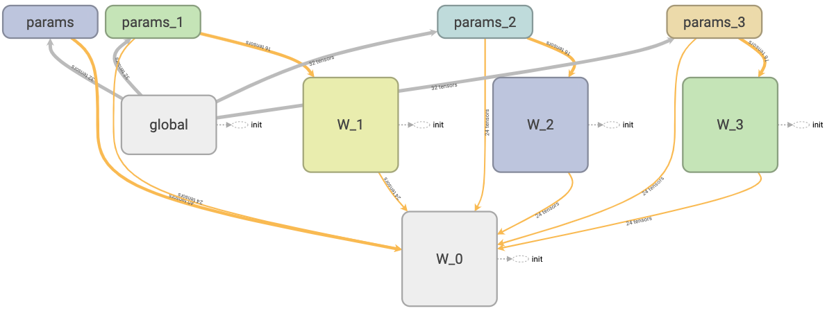
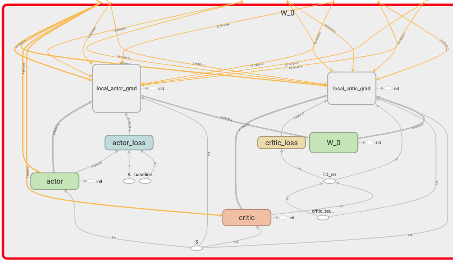
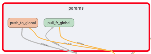
The ACNet class defines the models (Tensorflow graphs) and contains both the actor and the critic networks. The Worker class contains the work function that does the main bulk of the computation. A copy of ACNet is declared globally & it’s parameters are shared by the threaded workers. Each worker also have it’s own local copy of ACNet. Workers are instantiated & threaded in the main program.

ACNet class:

Loss function for the actor network for the discrete environment:

with tf.name_scope('actor_loss'):
    log_prob = tf.reduce_sum(tf.log(self.action_prob + 1e-5) * tf.one_hot(self.a, num_actions, dtype=tf.float32), axis=1, keep_dims=True)
    actor_component = log_prob * tf.stop_gradient(self.baselined_returns)
    # entropy for exploration
    entropy = -tf.reduce_sum(self.action_prob * tf.log(self.action_prob + 1e-5), axis=1, keep_dims=True)  # encourage exploration
    self.actor_loss = tf.reduce_mean( -(ENTROPY_BETA * entropy + actor_component) )                                        

Loss function for the critic network for the discrete environment:

TD_err = tf.subtract(self.critic_target, self.V, name='TD_err')
      .
      .
      .
with tf.name_scope('critic_loss'):
    self.critic_loss = tf.reduce_mean(tf.square(TD_err))

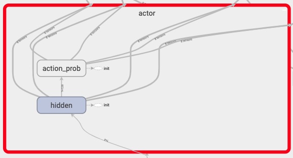
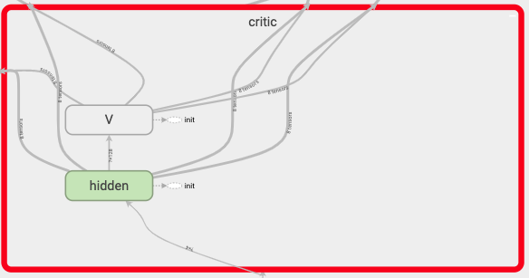
The following function in the ACNet class creates the actor and critic’s neural networks:

def _create_net(self, scope):
    w_init = tf.glorot_uniform_initializer()
    with tf.variable_scope('actor'):
        hidden = tf.layers.dense(self.s, actor_hidden, tf.nn.relu6, kernel_initializer=w_init, name='hidden')
        action_prob = tf.layers.dense(hidden, num_actions, tf.nn.softmax, kernel_initializer=w_init, name='action_prob')        
    with tf.variable_scope('critic'):
        hidden = tf.layers.dense(self.s, critic_hidden, tf.nn.relu6, kernel_initializer=w_init, name='hidden')
        V = tf.layers.dense(hidden, 1, kernel_initializer=w_init, name='V')         
    actor_params = tf.get_collection(tf.GraphKeys.TRAINABLE_VARIABLES, scope=scope + '/actor')
    critic_params = tf.get_collection(tf.GraphKeys.TRAINABLE_VARIABLES, scope=scope + '/critic')       
    return action_prob, V, actor_params, critic_params

Worker class:

Discounted rewards are used as critic’s targets:

critic_target = self.discount_rewards(buffer_r, GAMMA, V_s)

N-step returns are used in the computation of the Advantage function (baselined_returns):

# Advantage function
baselined_returns = n_step_targets - baseline

2 versions of N-step targets could be used:

• missing terms are treated as 0.

• use maximum terms possible.

Check this post for more information on N-step targets.

The following code segment accumulates gradients & apply them to the local critic network:

self.AC.accumu_grad_critic(feed_dict) # accumulating gradients for local critic  
self.AC.apply_accumu_grad_critic(feed_dict)

The following code segment computes the advantage function(baselined_returns):

baseline = SESS.run(self.AC.V, {self.AC.s: buffer_s}) # Value function
epr = np.vstack(buffer_r).astype(np.float32)
n_step_targets = self.compute_n_step_targets_missing(epr, baseline, GAMMA, N_step) # Q values
# Advantage function
baselined_returns = n_step_targets - baseline

The following code segment accumulates gradients for the local actor network:

self.AC.accumu_grad_actor(feed_dict) # accumulating gradients for local actor  

The following code segment push the parameters from the local networks to the global networks and then pulls the updated global parameters to the local networks:

# update
self.AC.push_global_actor(feed_dict)                
self.AC.push_global_critic(feed_dict)
    .
    .
    .
self.AC.pull_global()

The following code segment initialize storage for accumulated local gradients.

self.AC.init_grad_storage_actor() # initialize storage for accumulated gradients.
self.AC.init_grad_storage_critic()            

Check this post for more information on how to accumulate gradients in Tensorflow.

Main program:

The following code segment creates the workers:

workers = []
for i in range(num_workers): # Create worker
    i_name = 'W_%i' % i # worker name
    workers.append(Worker(i_name, GLOBAL_AC))

The following code segment threads the workers:

worker_threads = []
for worker in workers:
    job = lambda: worker.work()
    t = threading.Thread(target=job)
    t.start()
    worker_threads.append(t)
COORD.join(worker_threads)

Tensorflow graph:

References:

Asynchronous Methods for Deep Reinforcement Learning (Mnih, Badia, Mirza, Graves, Harley, Lillicrap, et al., 2016)

• 2020 10
• 2019 24